
Neuton.ai TinyML: A Dive Into Ultra-Compact, No-Code Edge AI for MCUs

Mikhail Seliadtsou
Sunday, November 30, 2025
Introduction
TinyML has become one of the most transformative trends in modern embedded development, enabling machine learning models to run directly on microcontrollers and ultra-low-power devices. Yet, building models small and efficient enough for real-world edge deployments is still a major challenge for most teams. Neuton.ai addresses this gap with a fully automated, no-code TinyML platform designed to generate extremely compact neural networks—often under 5 KB—without sacrificing accuracy or requiring model compression, pruning, or manual tuning.
In this article, we take a closer look at how Neuton.ai works, what makes its patented framework fundamentally different from traditional ML pipelines, and why it is quickly becoming a powerful tool for IoT and embedded engineers who need reliable, resource-efficient AI at the very edge.
Overview of Neuton.ai
Neuton TinyML is an automated no-code platform that empowers users to build extremely compact models and embed them into a wide range of devices, including the smallest 8-bit microcontrollers and even sensors. The platform has a patented neural network framework which is not based on any existing frameworks or non-neural algorithms. Neuton.ai automatically creates ultra-compact neural models (under 5 KB) with nearly the same accuracy, and runs them on almost any MCU without manual tuning or post-compression. Models of ~5 KB, inference up to ≈ 30× faster than TensorFlow Lite Micro on Arduino (example: Magic Wand use case). The tool is fully automatic, single iteration, no NAS, no manual tuning.
User guide declares that Neuton is absolutely free for developers worldwide.
NOTE: In-project documentation contains following notification, probably outdated:
If your account is on the Zero Gravity plan, the generated library will have a time limit for model inference. When creating a solution on the platform `neuton.ai`, you specified the frequency of data collection, then the limit will be about 30 minutes of inferences; if you did not specify, then the limit will be 1800 model inferences per power cycle of the device. For more information, please contact support@neuton.ai!
See more information in the official User Guide.
Training data preparation
Preparing training data is the most important stage of working with neural networks. The accuracy of the network largely depends on the quality and precision of data classification.
For example, let's take data from the project Sleep.Me - a sleep tracker. One of the device's functions is to determine the presence of a person in bed, after which the device begins to transmit data to the cloud, where a separate model determines the sleep phase. The device’s data consists of readings from 4 sensors, obtained every second. To train the model, this data needs to be converted into a CSV file suitable for Neuton .
Neuton has a pretty long list of data requirements, which can be found on the Dataset Requirements page. The main requirements are as follows:
A dataset must be a CSV file using UTF-8 or ISO-8859-1 encoding.
All column names (values in the CSV file header) must be unique and must contain only letters (a-z, A-Z), numbers (0-9), hyphens (-), or underscores (_).
In the case of sensor data from gyroscopes, accelerometers, magnetometers, electromyography (EMG), and other similar devices for creating models using Digital Signal Preprocessing, every row of a dataset should be device readings per unit of time with a label as a target. You should not shuffle signal labels or encode your signal for model creation.
For our training data, we will designate columns with sensor readings, as well as add 2 columns: sessionID and classification.
sessionID - differentiates data obtained during different experiments or on different devices. Training the model under various conditions and with different devices increases the model's accuracy, which positively affects the quality of the final product..
classification - is the most important parameter for training data, as it indicates how to classify the set of raw data; in our case, this is “binary classification” (a choice between two possible values “In bed” and “Out of bed”).
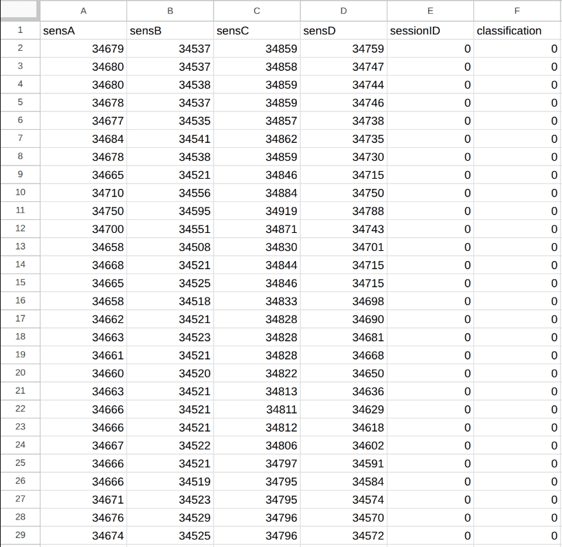
Example of training data
Model Creating
Solution Creation
The model creation process within Neuton always begins with creating a new Solution. The Solution is a workspace where you set up training parameters, manage results, and perform analysis.
To create a new Solution, click Add New Solution. A pop-up window titled “New Solution” will appear. Enter your desired Solution Name using Latin letters, and select the Task Type — Classification, Regression, or Anomaly Detection.
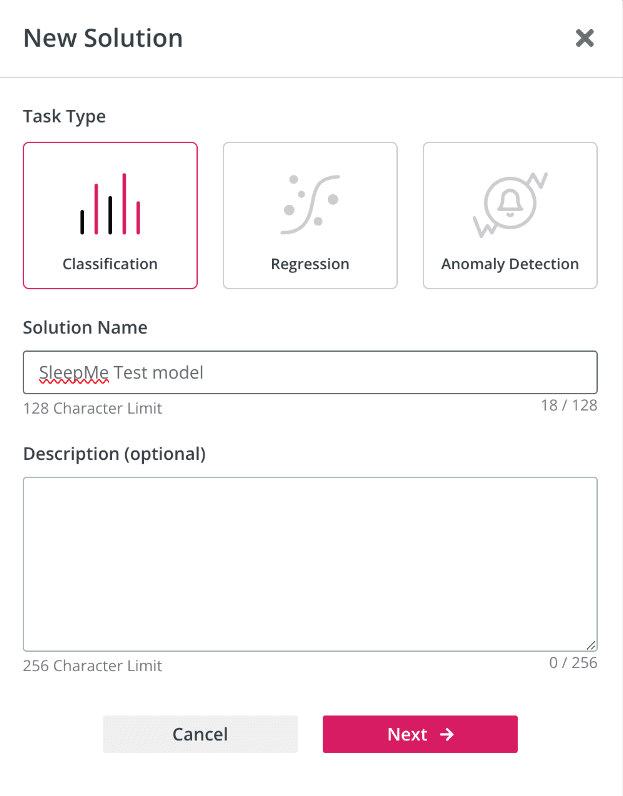
New solution window
Classification is the prediction of a target variable represented as a range of discrete classes. Binary classification tasks are represented by a target variable with two possible classes. Multi classification tasks are represented by a target variable with 3 or more classes.
Regression is predicting a continuous value (for example predicting the prices of a house given the house features like location, size, number of bedrooms, etc).
Anomaly detection is used to identify data points, events, or observations that deviate significantly from the norm or expected behavior within a dataset. These anomalies can indicate errors, fraud, or other unusual occurrences that warrant investigation.
We will use the classification type.
Data upload and setup
To begin model training, we first need to upload our dataset. Please ensure that data meets the Dataset Requirements before uploading.
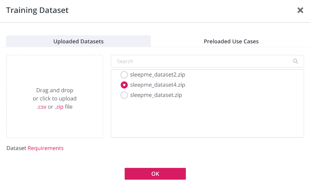
We can upload a new dataset, use previously uploaded data or use preloaded examples. Simply drag and drop the prepared CSV file.
After uploading training dataset, specify the target (classification) column and a Session ID column for time-series or session-based data. You may also exclude any features (columns) you consider irrelevant.
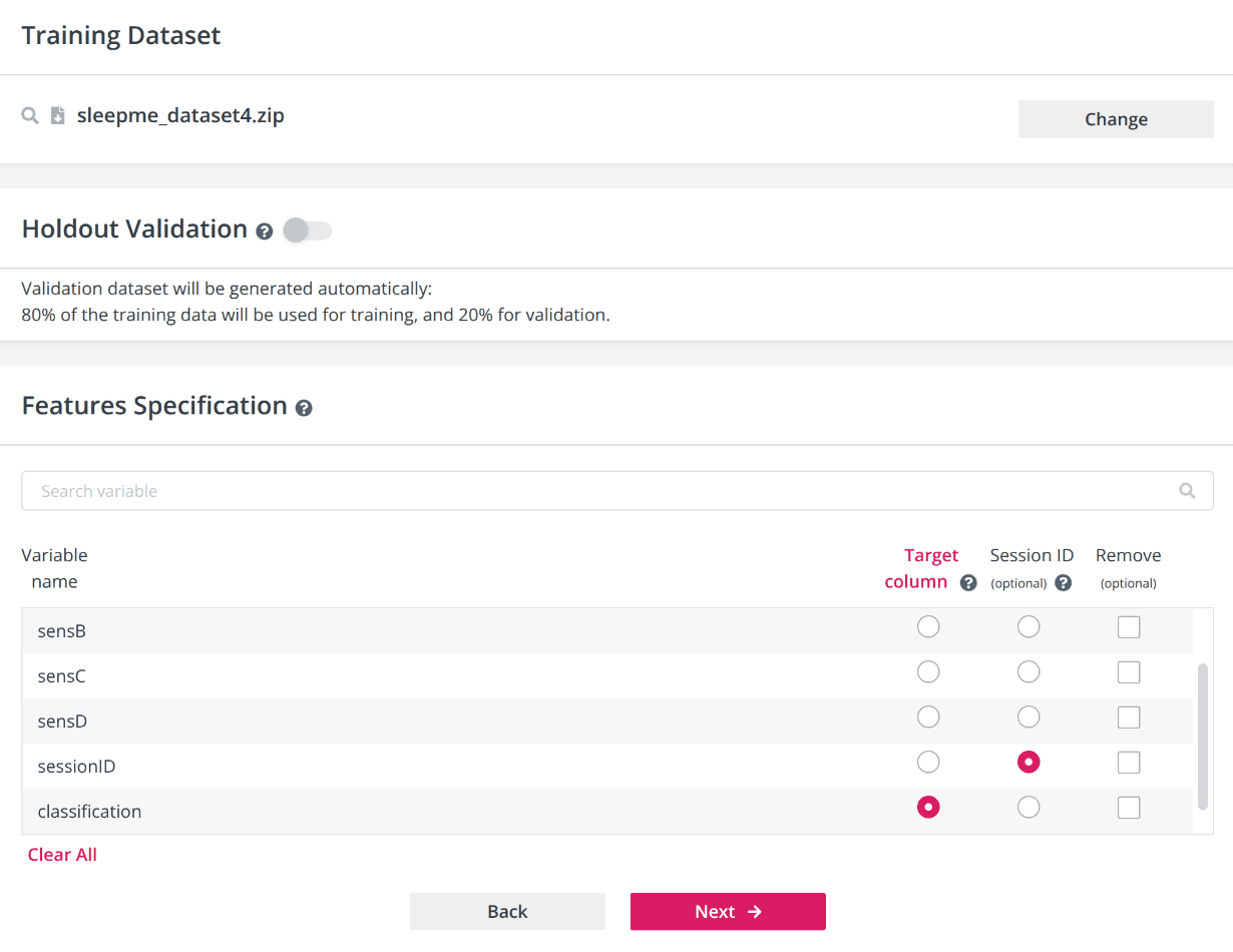
Choosing session ID and Target columns
To enable holdout validation, turn on the switch and upload your validation dataset. The holdout validation dataset must match the format of your training data. If you do not enable this option, the platform will automatically split your training dаta: 80% will be used for training, and 20% for validation. Holdout validation allows you to evaluate your model on a completely separate, user-provided dataset for more robust testing.
Model Settings
After we uploaded our dataset, proceed to configure the model settings. This step allows to define how the model will be trained and optimized for the specific task and hardware.
Let’s look at available settings closely:
Task type: Regression, Binary Classification, or Multiclass Classification and choose the metric to measure model quality. Neuton can auto-detect the task type based on the target variable, or it can be set manually. Default metric: Accuracy for classification, RMSE for regression.
During training, Neuton tracks the validation metric on the dedicated validation dataset at each iteration. Training automatically stops before overfitting occurs, based on the results from this validation set. The platform computes all available metrics for the selected task type.
Model coefficients and weights: 8-bit, 16-bit, or 32-bit. Lower bit depths (8 or 16) help minimize model size and optimize device resource usage. For 8 and 16-bit storage, calculations can be performed in both floats and integers; for 32-bit, only floats are used. By default, this setting matches the dataset type, but it can be adjusted as needed.
Activation functions: Floating-point or Quantized. For 32-bit weights, only floating-point activation is available. To achieve the smallest model footprint, select 'Quantized Activation' when using 8- or 16-bit quantization-aware weights.
Output format: Quantized (integer) or Floating-point. Options:
Quantized 8-bit: probabilities from 0 to 255
Quantized 16-bit: probabilities from 0 to 65,535
Floating-point 32-bit: probabilities from 0 to 1
Quantized format is only available when quantized weights & coefficients are selected. For 32-bit (floating-point) weights, only floating-point output is available and cannot be changed.
Data type: data type for all features in your training dataset: INT8, INT16, or FLOAT32. For mixed-type datasets, choose the widest type present (e.g., FLOAT32 if any value is a float). Correct selection reduces device memory use and inference time.
Normalization type: Unique scale for each feature (increases accuracy, may increase model size) or Unified scale for all features (reduces size if values are already on the same scale).
Training Stop Options: Control model complexity and training time using these options:
Maximum Number of Coefficients: Limit the number of coefficients in the model (by default, unlimited).
Maximum Training Duration (hours): Limit training time. The best model will be saved automatically if the time limit is reached.
Maximum Value of Evaluation Metric: Training will stop once the specified metric value is reached (if achievable for your data).
Target Hardware: Select one or more hardware targets for model deployment. Supported options include Cortex M0, Cortex M4, Cortex M33, STMicro ISPU, and Microchip-8 series. The platform will optimize model conversion and code generation for the selected hardware.
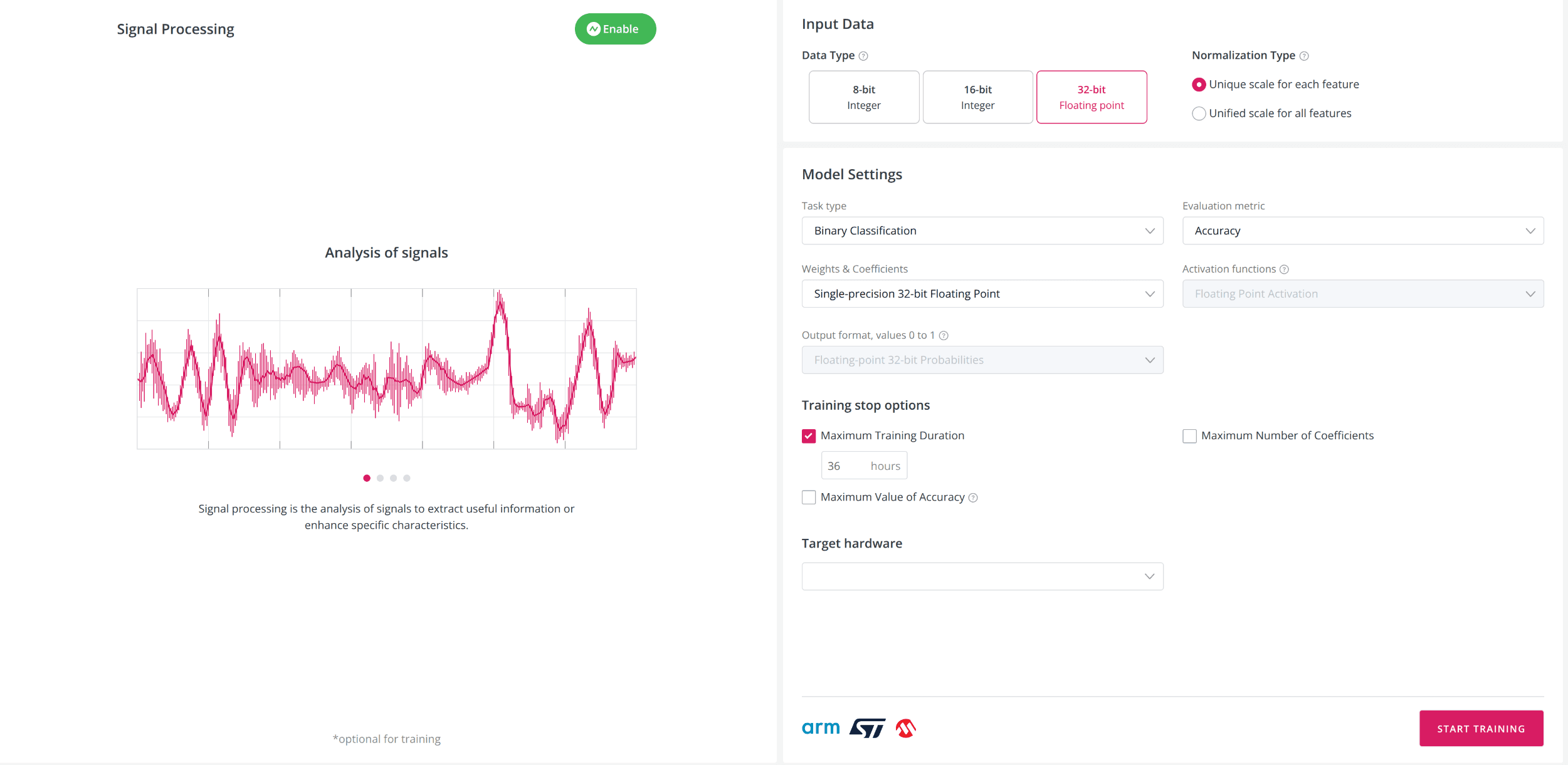
Signal processing
Signal Processing (SP) enables automatic processing of raw sensor data and extraction of features for datasets from gyroscopes, accelerometers, magnetometers, EMG, and similar sources.
Signal processing could be set manually or with a wizard. The wizard will walk you through a series of questions and automatically configure all required SP settings: windowing parameters and the list of features to extract. This is the fastest way to get started if you are new to signal processing.
Let’s look at manual settings.
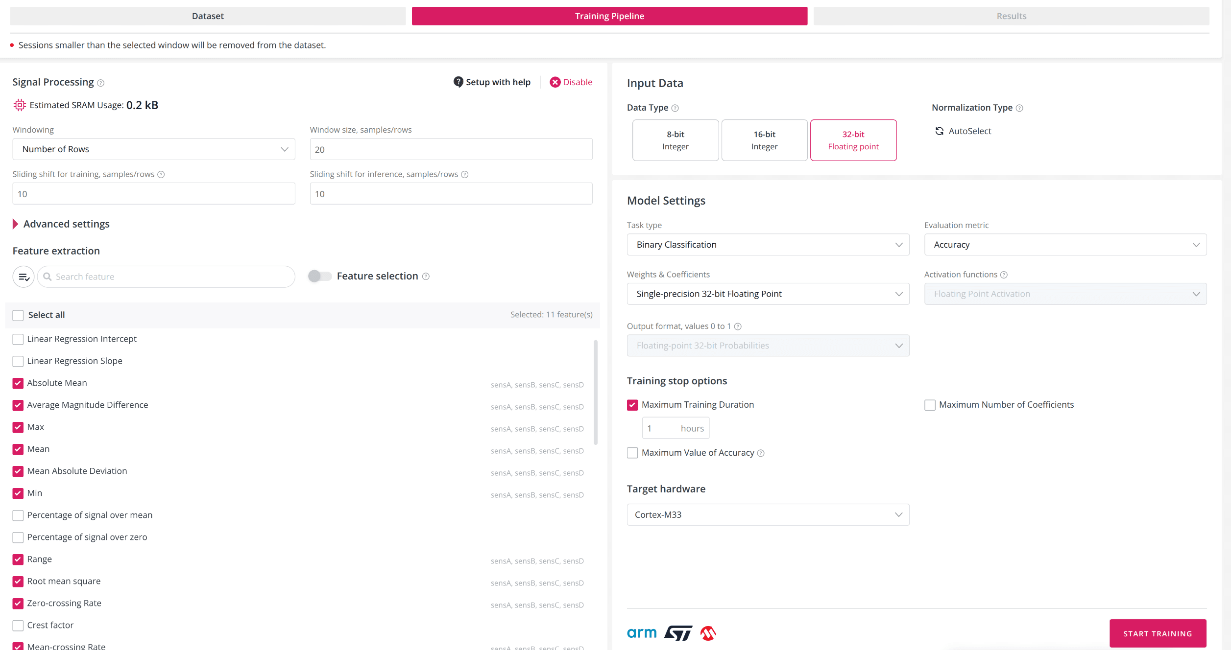
Manual settings for Signal Processing
Windowing: converts a sequential signal data into vectors for feature extraction. Window size is the chunk of data used for each step. For correct model training, ensure both training and validation datasets are brought to the same window using upsampling or downsampling, before uploading to the platform. Recommended window size: from 5 samples/rows up to 1000 samples/rows.
Window size could be specified in three ways:
Time interval: Set window size in milliseconds (ms) and frequency in Hertz (Hz). The platform will automatically convert this to a number of samples. For multiple sensor frequencies, downsample or upsample first.
Number of Rows (Samples): Set the exact number of samples for the window.
Auto Determination: (for classification and regression) The platform will automatically choose the optimal window size using a built-in algorithm. You may specify min/max window size boundaries and sliding shift in %.
Sliding Shift: determines window overlap - how many samples to shift for the next window. If shift = window size, there is no overlap. Available for both training and inference.
Estimated SRAM Usage: The platform estimates SRAM usage based on your selected window size and features. Actual usage will be determined after model training and compilation. For window auto-determination, SRAM estimation appears only after training.
Feature Extraction: When the window size is set, the platform automatically extracts selected features for each column (variable/axis). The same features are extracted during inference. You can enable/disable features, use the “Edit” button, “Select All”, or restore defaults. The search bar lets you quickly find features.
Feature Selection: Feature Selection allows you to automatically select the most important features for model building, reducing dataset size and improving performance. Features will be removed if:
They are constants
Their correlation with other features is 1.00
They cause a metric loss of ≥ 0.875% (Feature Importance)
After setting up all the parameters press the START TRAINING button and wait for results. Depending on the amount of input data and the complexity of the final model, the process can take anywhere from a few minutes to several hours..
Model training results
After starting the model training, we will be redirected to the “Results” tab.
Note: Sometimes the "Results" tab may display incorrectly upon reaching 100%, it is necessary to return to the "My Solutions" page and reopen the solution.
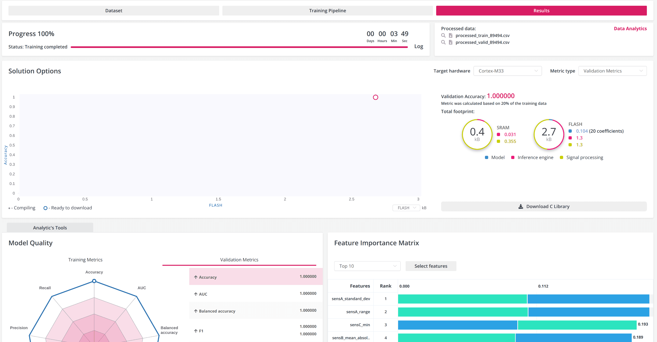
Common view of the Results page
Solution Options: This chart presents iterations of growth and model construction on a single graph. With this feature, it is possible to compare, choose, and download models with differences of up to kilobytes in size and hundredths of a percent in accuracy, making it possible to embed these models in the most resource-constrained devices. (Watch the video to learn more)
Processed data: You can see what data the model was trained on, taking into account the additional settings you have chosen, for example, features created from Feature Extraction. By clicking on the "Data Analytics" button, you can access an overview of the analytics charts based on the processed data.
Model Info Area: Displays information related to the model that has been selected in the model growth chart.
Info area contains:
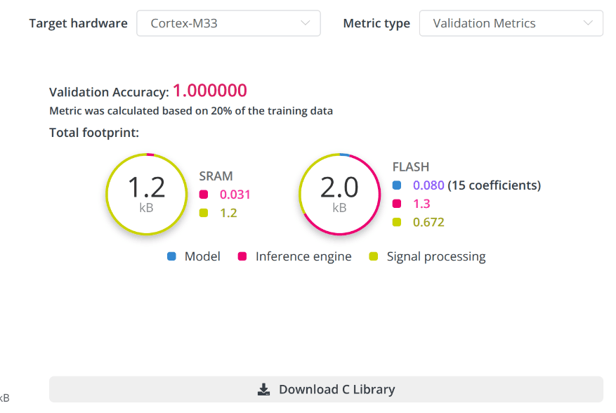
The target metric value and its name. Two types of metrics are displayed: cross-validation and holdout (provided the holdout dataset was used prior to training). To switch between different metric types, use the switch located in the chart area.
The total footprint of the selected model. Here you can find information on the estimated usage of SRAM and FLASH memory by the model, inference engine, and signal processing. Estimated values are provided for the target hardware selected. (these values are provided as an example). After completing the training, C libraries will be prepared for a wider range of hardware types, and source code will be available for enterprise plans.
The “C Library” button for the selected model, that allows users to download the resulting model and code for inference on the device.
Analytics Tools: This tool automates processed data (training dataset) analysis and relation to the target variable. The report is generated during model training for each solution. Given the potentially wide feature space, up to 20 of the most important features with the highest statistical significance are selected for data analysis based on machine learning modeling. The data analysis tool is available on the “My Solution” page and the “Results” tab, found via the “Data Analysis” button.
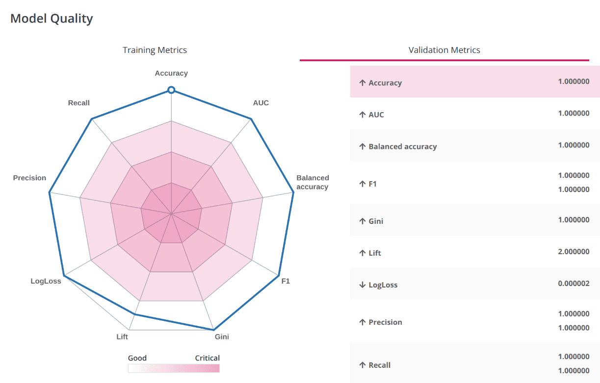
Model Quality Diagram
The Model Quality Diagram simplifies the process of evaluating the model quality. The values of all metrics are evaluated on a scale from 0 to 1, where 1 is the most accurate model. It also allows users to understand metric balance for the selected model. When the figure displayed is close to the shape of a regular polygon, that conveys a perfect balance between all metric indicator values.
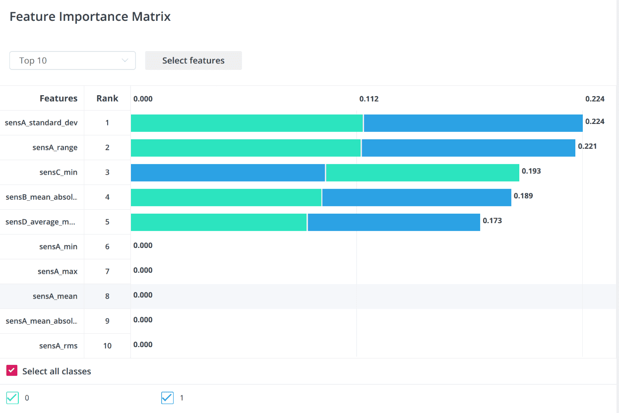
Feature Importance Matrix
After the model has been trained, the platform displays a chart with the 10 features that had the most significant impact on the model prediction of the target variable (for the selected model). The chart can be found in the Results tab. The Feature Importance Matrix helps to evaluate the impact of features on the model. If the feature does not affect the model at all (normalized value = 0), then you can exclude this variable from building the model.
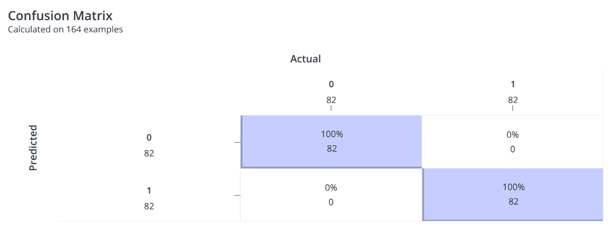
Confusion Matrix
The Confusion Matrix shows the number of correct and incorrect predictions based on the validation data for the selected model.
Test data analysis
In the images above, you can see that training the model for Cortex-M33 took less than 4 minutes. The platform prepared only one model with an excellent accuracy of 1.0, and all checks from the Validation data were passed flawlessly.
However, such perfect output indicates that the data for training and validation were too uniform and the amount of data was too small. Let's pay attention to the Feature Importance Matrix graphs, where the greatest contribution comes from the values of sensor A. For example, let's look at the graphs of one of the example datasets.
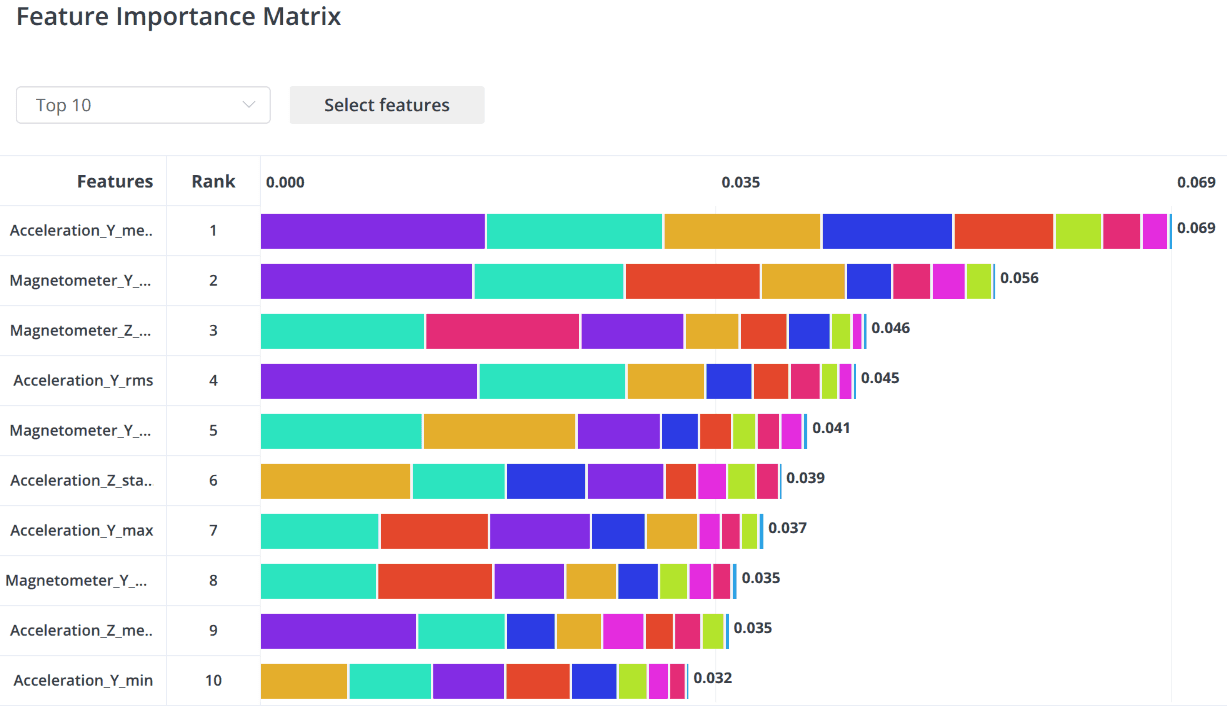
Feature Importance Matrix from an example dataset
Quality data preparation is the main key to building a successfully functioning model. The more diverse and extensive the data prepared, the better. For example, data from Sleep.Me was obtained from one device and one sleeping place; to improve the quality of the sample, it is necessary to add data collected for different positions of the lying person: on their back, on their side, on their stomach; from different surfaces, such as a sofa and the floor.
Model usage
On the results tab there is a button “Download C Library”. The archive contains the following folders and files:
artifacts – contains models converted to various formats, as well as an executable file for predictions on the desktop.
neuton – contains libraries for embedding.
neuton-generated – contains information necessary for the correct operation of libraries.
LICENSE – contains the possibilities and restrictions on the use of Neuton’s intellectual property.
README – contains instructions for leveraging libraries.
Model check
Neuton Inference Runner is an executable containing a user-specific Neuton ML solution. With its help, the user can validate the results of the inference of the model even without implementation in the Edge device. Windows, Mac and Linux are supported.
Neuton Inference Runner has user CLI interface for executing various commands. To see help you can run neuton_inference_runner without any arguments:
Use inference command to run inference on the provided CSV dataset. Supported two kinds of datasets: CSV text file format and Neuton dataset binary file format (with corresponding filename extensions '.csv' and '.bin'). The CSV dataset should have a header and contains only number fields separated by comma. Inference result will be printed to the screen. Additional params -s filename (or --save filename ) stores the inference results to the CSV file. Usage examples:
Run Inference on the MCU
There are only two folders that should be added to a project for integrating Neuton:
neuton - main framework folder in which all Neuton algorithms, utilities, are located;
neuton_generated - folder containing all user solution-specific files (neural network model, data preprocessing configuration, etc).
Also, add folder where ./neuton_generated is located and ./neuton/include folder to the project INCLUDE paths.
Next, include the main header file of Neuton:
For making an inference with Neuton, there are only 3 functions that should use:
neuton_nn_setup - Set up the internal components of Neuton, should be called first and once;
neuton_nn_feed_inputs - Feed and prepare live input features for model inference;
neuton_nn_run_inference - Run live input features into a Neuton machine learning algorithm (or “ML model”) to calculate an output;
To feed input values make an array with model raw input features(signal data). Inputs count and order should be the same as in the training dataset.
Pass this input array to the neuton_nn_feed_inputs function.
In case the Neuton solution needs to collect a data window, the following sample-by-sample feed algorithm could be used:
Or feed all input samples at once:
When input buffer is ready for running inference, call neuton_nn_run_inference with three arguments:
p_input - Input features for model inference, obtained from @ref neuton_nn_feed_inputs() API call
p_index - Index of predicted target(class) with highest probability;
pp_outputs - Pointer to pointer to the internal buffer with all predicted outputs, contains predicted target variable (for regression task) or probabilities of each class (binary/multi classification tasks).
Example code
Inference results are encoded (0…n). For mapping on own classes, the dictionaries could be used:
binary_target_dict_csv.csv - bynary classification task;
multi_target_dict_csv.csv - multitarget classification task.
Conclusion
Neuton.ai brings a new level of practicality to TinyML, allowing developers to generate ultra-compact neural models that run directly on microcontrollers and low-power IoT devices. Its automated, no-code approach removes the complexity of traditional ML workflows and makes true edge intelligence accessible for a wide range of applications.
As companies increasingly shift toward on-device processing and smarter embedded products, expert guidance becomes essential. Iomico supports organizations with both consultancy and hands-on implementation of Edge AI, helping teams prepare data, integrate TinyML models, and deploy reliable AI-enabled devices efficiently.
If your company is exploring TinyML or edge intelligence, Iomico can help you build and deliver solutions that are accurate, efficient, and production-ready.


