Bluetooth Channel Sounding in the Real World: nRF54L15 Field Test Results

Bluetooth Channel Sounding promises accurate distance measurement over a standard Bluetooth Low Energy link. Vendor demos look great, but how does it behave when a body blocks the antenna, when the street is full of people and metal, or when one device is moving? We took two pairs of nRF54L15 boards outdoors and measured it, from 1 m to 100 m.

Key findings

• Clear line of sight (3–100 m): after per-antenna calibration, the fused estimate averaged −0.02 m error with the nRF54L15 DK PCB antenna and −0.14 m with the nRF54L15 Tag chip antennas. These are calibration results, not an independent validation.

• Busy street, static devices: RMSE of 2.1 m (DK) and 2.8 m (Tag) between 3 m and 10 m, rising to 6.9 m for the DK across 3–70 m.

• Moving device: RMSE of 3.2 m (DK) and 5.1 m (Tag) up to 10 m, but 25.9 m beyond 30 m for the DK, with a strong underestimation bias.

• Availability: at a 5 Hz target rate, only 69.5% (DK) and 58.6% (Tag) of measurement slots produced a distance in line of sight, and 20.6–63.0% in every other scenario.

• Calibration does not travel: fusion weights tuned in line of sight made the fused result worse than RTT alone once the device was moving in a harsh environment.

Context

Since 1998, the Bluetooth Special Interest Group (SIG) has been developing Bluetooth, a wireless standard initially intended for short-distance communication between two devices. Today, depending on the PHY and radio design, Bluetooth links can reach hundreds of meters under optimal conditions, and devices are no longer limited to point-to-point links: they can form a mesh of many interconnected nodes.

In 2024, the Bluetooth SIG published the Bluetooth 6.0 specification, and with it Bluetooth Channel Sounding (B-CS), which gives applications built on top of it the ability to measure distance.

What Is Channel Sounding?

Channel sounding is not a new concept introduced by the Bluetooth SIG. In telecommunications theory, the term has long described the process of probing and characterizing a communication channel (wired or wireless) so that nodes can negotiate output power, coding and every other aspect of the communication efficiently.

Goal of This Test

The goal of this article is to show how well this new technology performs in practice. We ran a series of tests to answer one question: can Bluetooth Channel Sounding accurately measure distance in a harsh environment?

How Bluetooth Channel Sounding Works

Initiator and Reflector

The device that starts the ranging process is called the Initiator; the second device is called the Reflector.

Channel Sounding Modes

Bluetooth Channel Sounding uses modes to define the purpose of each Channel Sounding step. A step can exchange synchronization packets, Channel Sounding tones, or both, depending on its mode. Channel Sounding itself does not calculate distance: the application does, using the phase and timing information Channel Sounding provides.

• Mode 0 – FFO calibration. Determines the Fractional Frequency Offset (FFO) between the frequency generation of the two devices. It is used to compensate the phase and timing measurements and does not provide a distance estimate on its own.

• Mode 1 – Round-Trip Time (RTT). The Initiator sends a synchronization packet and the Reflector replies after a negotiated, known turnaround time. After compensating for that turnaround time and implementation delays, the remaining round-trip propagation time gives the distance.

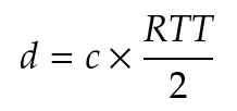
• Mode 2 – Phase-Based Ranging (PBR). Initiator and Reflector exchange Channel Sounding tones across multiple radio channels. Channel Sounding defines 1 MHz-wide channels, 72 of which are available for this purpose, although a single procedure does not have to use all of them. The measured phase difference versus frequency reveals the propagation delay.

• Mode 3 – Combined RTT and PBR. Exchanges both synchronization packets and tones, so RTT and PBR data are collected in the same step. Support for Mode 3 is optional.

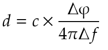
This is a simplified explanation, and these formulas are only some of the options an application can use to infer distance from the phase and timing data that Channel Sounding provides.

Test Hardware

We ran the tests on Nordic Semiconductor nRF54L15-based kits: the nRF54L15 DK, which uses a PCB antenna, and the nRF54L15 Tag, which uses chip antennas. This let us compare the two antenna types. PCB antennas trade a larger footprint for lower cost and greater reach compared with chip antennas.

A smartphone can act as a Channel Sounding Reflector, but to assess antenna performance properly both devices in each pair had to use the same antenna. We therefore used two DKs and two Tags.

nRF54L15 DK. Image: Nordic Semiconductor.

Test Plan

For every test we used the Channel Sounding ranging samples (ras_reflector and ras_initiator) from nRF Connect SDK (NCS) v3.4.1, with a small modification to collect the samples. We ran four tests:

• Controlled Line of Sight and antenna calibration (CLOS).

• Static Body Blocking (SBB).

• Static Harsh Environment (SHE).

• Dynamic Harsh Environment (DHE).

To collect data, the Initiator wrote its distance estimates into its Bluetooth advertising payload. A simple BLE mobile app sampled those advertisements and saved them to a CSV log.

Methodology and Statistics

Channel Sounding provides raw data, and the application has to choose an algorithm to estimate distance. We used the three estimators provided by NCS: IFFT, Phase Slope (PS) and RTT. For every received sample, knowing the real distance of the test point, we calculated the signed error.

Signed Error

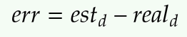
The error is the distance reported by an estimator minus the known real distance, calculated for each sample and each estimator. A positive error means the estimator overestimates the distance; a negative error means it underestimates it.

Calibration (Bias)

The calibration offset for each estimator was calculated as the sample-weighted average signed error across all valid samples in the CLOS scenario:

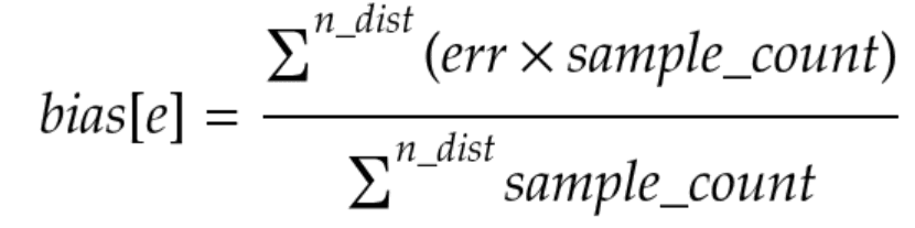
This bias is the offset that depends on the antenna and the configuration: it shows how far, on average, an estimator was shifted from the known real distance during calibration. The corrected distance used by the application is then:

Calibration is necessary because the RF path is different for every antenna. Board layout, antenna type, PCB traces and radio configuration can all introduce their own systematic error. That is why the nRF54L15 Tag and the nRF54L15 DK each have their own stored calibration values, and why changing the radio configuration requires a new calibration.

Fused Estimate

The CLOS tests showed that the estimators behave differently depending on distance, so we combined them into one estimate. Each estimator is weighted by the inverse of its squared RMSE:

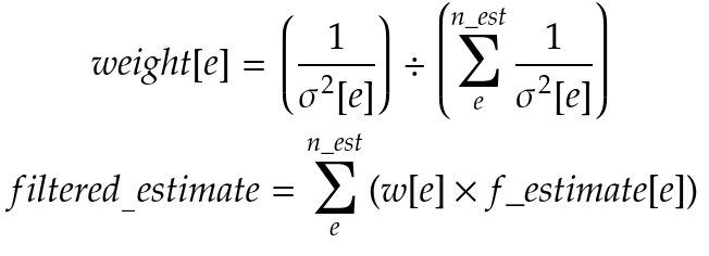
The filtered (fused) distance is a weighted average of IFFT, PS and RTT. If an estimator is unavailable, only the valid estimators are used and their weights are normalized again.

Availability

Availability was calculated from the device timestamps. At a 5 Hz rate, one measurement is expected every 200 ms, and availability is the share of those scheduled slots that actually produced a valid filtered distance:

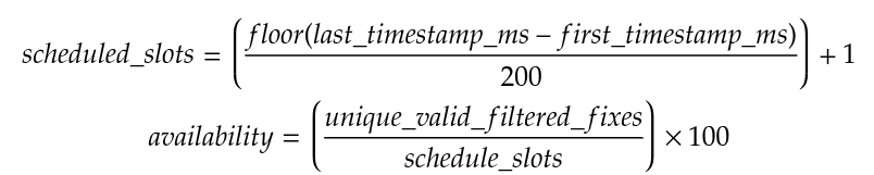
This distinction matters. A result is not good only because its average error is low: if the device cannot deliver measurements at the expected rate, the system may be unsuitable even when the measurements it does deliver are accurate.

Radio Configuration

In all tests, the Initiator and Reflector used the same Channel Sounding configuration. An ACL connection was used to negotiate and control the Channel Sounding procedures. For the coded PHY configurations, we kept the ACL connection on the 1M PHY and used the coded PHY only for the Channel Sounding procedure. This was the most stable approach we found.

Test 1: Controlled Line of Sight and Antenna Calibration

This is the best-case test. It was run in an open space with no objects in the direct path between the devices and no nearby metal surfaces that could cause significant reflections. The goal was to understand how the estimators behave when the propagation path is as benign as possible.

We ran one campaign with two nRF54L15 Tags (dual chip antennas) and another with two nRF54L15 DKs (PCB antennas). One device acted as Initiator and the other as Reflector. The devices were placed at known distances of 3, 5, 7, 10, 20, 30, 40, 50, 60, 70, 80, 90 and 100 m and stayed static while estimates were collected at each point.

The CLOS test used the coded PHY S8 configuration and a 5 Hz measurement rate, so a distance estimate was expected every 200 ms. This let us evaluate both the estimates received and the estimates that were missing (availability).

The same CLOS data was used to calculate the offsets and estimator weights. These results therefore show how the calibrated configuration behaves in its own calibration environment and should not be read as an independent validation of accuracy. The body-blocking and harsh-environment tests show how it behaves in more realistic conditions.

Results

Availability

PS did not produce calibration samples at 80 m, 90 m or 100 m for either antenna profile.

Bias, RMSE and Fusion Weights

Average Error (m)

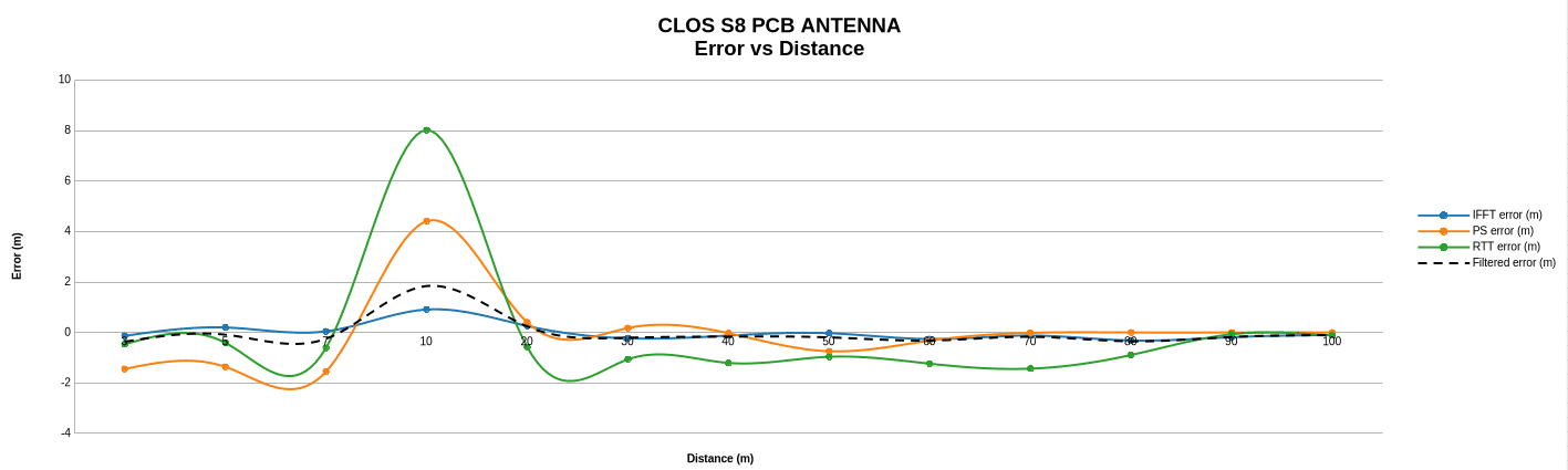
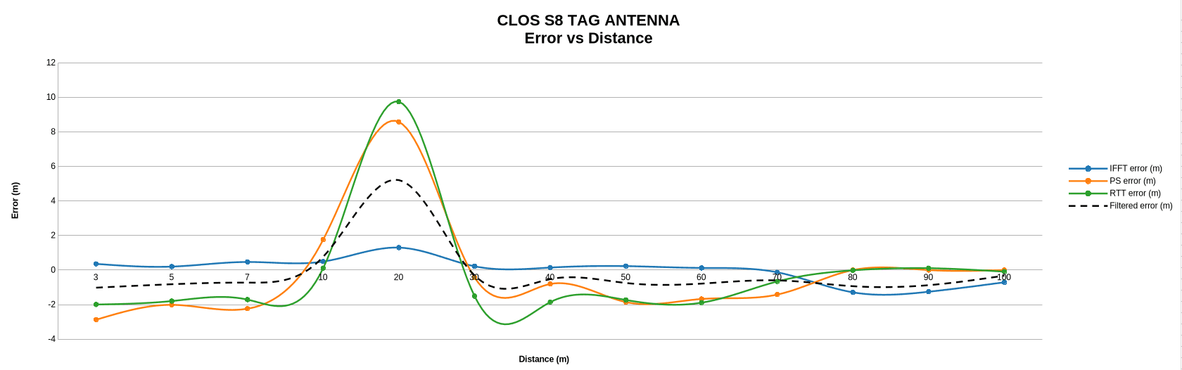
The following two charts show the error versus distance after calibration (bias subtracted) for both antennas.

Average Variance (m²)

Received RF Power vs. Distance

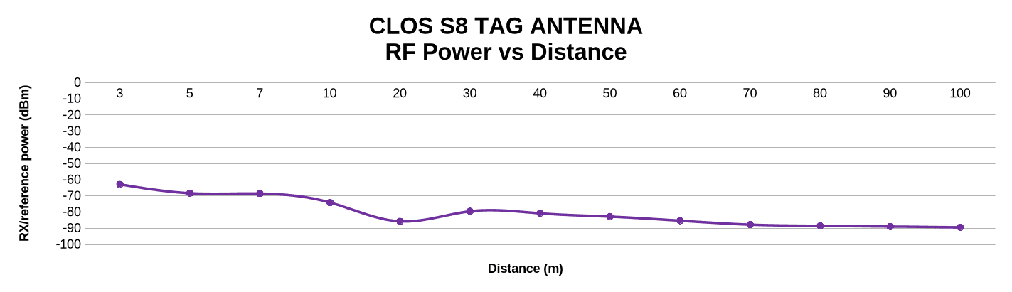
In line of sight, the DK PCB antenna received roughly −50 dBm at 3 m and about −77 dBm at 100 m. The Tag started lower, at about −63 dBm at 3 m, and dropped to about −89 dBm at 100 m.

Test 2: Static Body Blocking

Next, we looked at what happens when a human body partially or completely blocks the direct radio path. The devices were kept static at known distances, as in CLOS, but a person's position was changed to block one or both antennas. This is a much harder radio condition because the body absorbs, reflects and attenuates the 2.4 GHz signal.

We used the same two antenna configurations, the same coded PHY S8 configuration, 7 dBm transmit power and the 5 Hz reference rate. The calibration offsets and fusion weights from the corresponding CLOS campaign were applied to the raw IFFT, PS and RTT estimates before calculating the filtered distance.

We evaluated three blocking configurations:

• Reflector blocking: a person blocked the Reflector antenna while the Initiator antenna was unobstructed.

• Initiator blocking: a person blocked the Initiator antenna while the Reflector antenna was unobstructed.

• Both blocking: both the Initiator and the Reflector antennas were blocked.

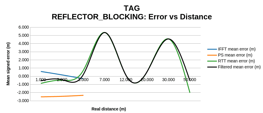
The DK campaign used distance points of 1, 2, 3, 7, 12, 20, 30, 50, 70 and 100 m. The Tag campaign did not achieve the same coverage: its received samples reached 50 m, and the both-blocking case only reached 20 m. This is a result in itself, because missing samples are part of the behavior we need to measure.

As in CLOS, the system was expected to provide a new estimate every 200 ms. The mobile logger received the estimates advertised by the Initiator, and duplicate advertisements were removed using their sample index.

This test separates a value being received from a value being useful. An estimate can be numeric yet have a large error, and a configuration can produce acceptable individual estimates while leaving long gaps with no new measurement. We therefore evaluated body blocking with error metrics, received signal power and availability.

The body-blocking datasets have an important limitation: the number of samples is not uniform across distances and configurations. Some far-distance points, especially in the both-blocking configuration, contain a single received sample. Those points show that the link or estimator was affected, but they cannot support meaningful variance or percentile statistics. The body-blocking test shows the degradation caused by obstruction; it does not by itself establish a reliable static operating range.

Results

Availability

The DK had its best availability when only the Initiator was blocked. Blocking both devices cut its availability to 20.60%: the two obstructions affected not only the estimated distance but also the ability to deliver a new estimate at the expected 5 Hz rate. The Tag shows low availability in every configuration. Its both-blocking figure should be read with care: it represents only 23 valid samples from a short, incomplete capture.

Filtered Estimate Error

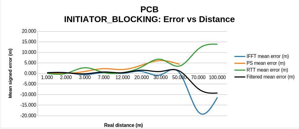
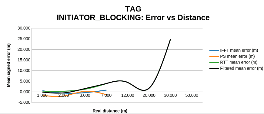
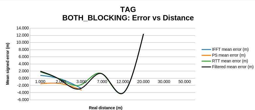
These pooled figures should not be read in isolation. A few far-distance outliers inflate the DK reflector-blocking RMSE, and the Tag both-blocking set is too sparse to cover a complete distance range. Still, the values show that the CLOS calibration and fixed fusion weights did not fully compensate for the changes introduced by body blockage.

Error vs. Distance

The following charts show the DK and Tag errors after applying the corresponding CLOS calibration offsets, making the difference between blocking the Reflector, the Initiator and both devices visible. High-distance points with a single received sample are descriptive only.

Received RF Power

For both antenna profiles, blocking both devices produced the weakest average received power, and the Tag started from a lower power level in every configuration. RSSI alone does not predict every ranging error, but together with the availability results it shows how body absorption and orientation degraded the radio path.

Test 3: Static Harsh Environment

The static harsh-environment test moved away from the controlled conditions of CLOS. The Initiator and Reflector stayed static at known distances, but this time on a city street with people moving around, metal objects, other radio systems and many possible reflections. The goal was to see how the same calibrated configuration behaves when the radio channel is no longer clean and predictable.

Test line along the avenue. Map data © Google.

Again, we ran one campaign with the nRF54L15 Tags and another with the nRF54L15 DKs, both with coded PHY S8, 7 dBm transmit power and the 5 Hz reference rate. The raw IFFT, PS and RTT estimates were corrected with the offsets from the corresponding CLOS campaign, and the same fixed weights were used to calculate the filtered distance.

The devices were placed at known static distances between 3 m and 70 m. Most measurements were collected between 3 m and 30 m; the farther points contain fewer samples. At every distance the application advertised the raw estimator outputs, the device timestamp and the received power, and the mobile logger removed repeated samples using the sample index.

Because the real distance was known, we could calculate signed error, absolute error, RMSE and percentiles for every estimator and for the filtered estimate. We also recorded the received power of the Reflector's signal, so we could check whether a weak signal was linked to growing error or missing estimates.

Availability was calculated as in the previous tests. A received numeric value does not mean the system was measuring continuously, which matters in a harsh environment: an estimate can be accurate at one moment while the next ones are delayed or lost because of interference or a change in the propagation path.

This test also exposes a limitation of fixed calibration. The offsets correct the systematic error observed during CLOS, but they cannot remove new errors caused by multipath, attenuation or interference. Likewise, the estimator weights come from controlled CLOS data: they can improve the average estimate, but they are not necessarily optimal when the environment changes.

Results

Availability

Every estimate received from the Initiator had a numeric filtered value, yet many expected 200 ms slots produced no new estimate at all. Counting received samples alone is not enough to describe the system's behavior.

Filtered Estimate Error

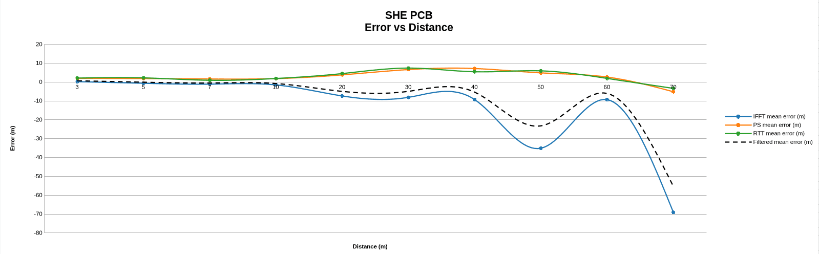
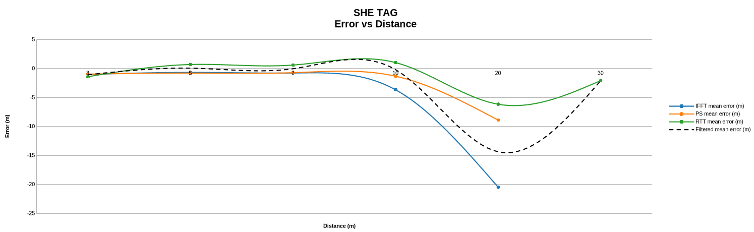
The negative mean signed error at longer distances means the filtered output underestimated the real distance, especially for the DK from 20 m onwards. The Tag capture has few far-distance records, so its 20 m and 30 m results are useful as diagnostics but carry less confidence than the well-populated close-range points.

Error vs. Distance

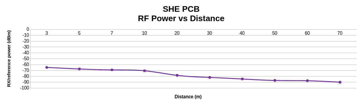
The charts below show the mean error after applying the CLOS calibration offsets. IFFT starts to underestimate the distance as conditions get harder, and the filtered estimate follows, because IFFT carries the largest fixed fusion weight for the DK PCB antenna.

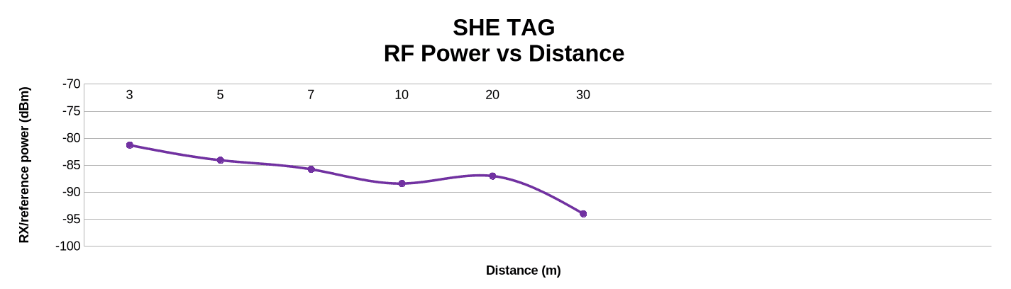
Received RF Power vs. Distance

The Tag received weaker power from the very first distance, and both profiles lost power as separation increased. This trend is related to the measured error but does not fully explain it.

Test 4: Dynamic Harsh Environment

The dynamic test added movement to the previous scenario. The Initiator stayed at a reference location while the Reflector was carried through the same outdoor environment. Because the distance between the devices kept changing, it could not be used as a known test point the way it was in the static tests.

We therefore ran the mobile logger and a GPS logger at the same time. The mobile app stored the distance estimates advertised by the Initiator together with the phone and device timestamps; the GPS log stored its own position and timestamp. In post-processing, every Channel Sounding record was matched to the closest GPS timestamp. If the time difference was larger than half a second and the record fell between two GPS points, linear interpolation was used to obtain the GPS distance.

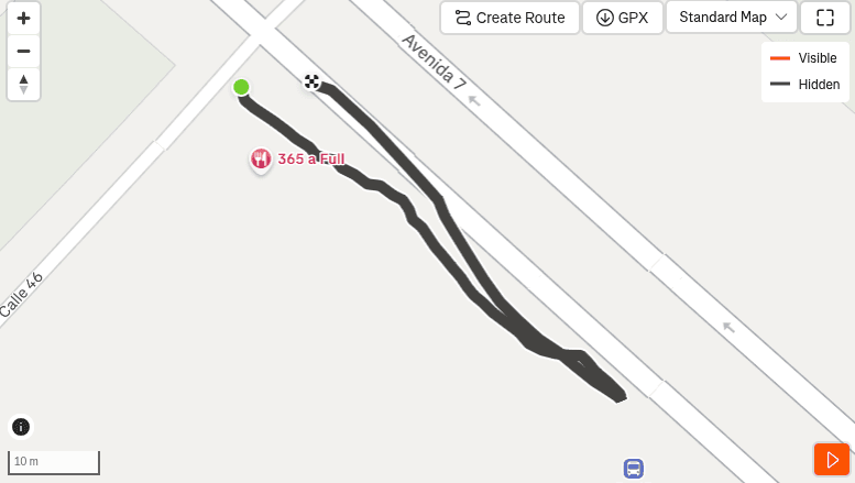
We used the same coded PHY S8 configuration, 7 dBm transmit power and 5 Hz rate. The DK campaign was repeated twice and the Tag campaign three times. The CLOS calibration offsets and fixed weights for each antenna were applied before comparing the filtered estimate with the GPS-derived distance.

Because every record can have a different distance, orientation and propagation path, the measurements were grouped into distance bands during analysis rather than by fixed test points. This let us calculate error, received power and availability while the Reflector moved away from and back towards the Initiator.

Timestamp synchronization also became critical: a good distance estimate matched to the wrong GPS time would look like an error even if the ranging was correct. Records outside the GPS time range were therefore excluded from the error calculation, though they were still used to evaluate availability and capture coverage.

Finally, the dynamic test made it clear that observed reach and usable ranging reach are different things. A device can stay connected and keep advertising a numeric estimate at a given distance while that estimate already has a large error or arrives too infrequently. The two antenna campaigns also followed different paths and produced different numbers of records, so their farthest received points are not a direct antenna comparison. The dynamic results are most useful for showing how calibrated estimators with fixed fusion weights react to a changing real environment.

Results

Availability

Dynamic availability stayed well below 100%, even though nearly all GPS-aligned records contained a numeric filtered estimate. The Tag campaign had one GPS-aligned record at 30.607 m with no numeric estimator value, which is why it has 93 records but 92 valid filtered estimates.

Filtered Estimate Error

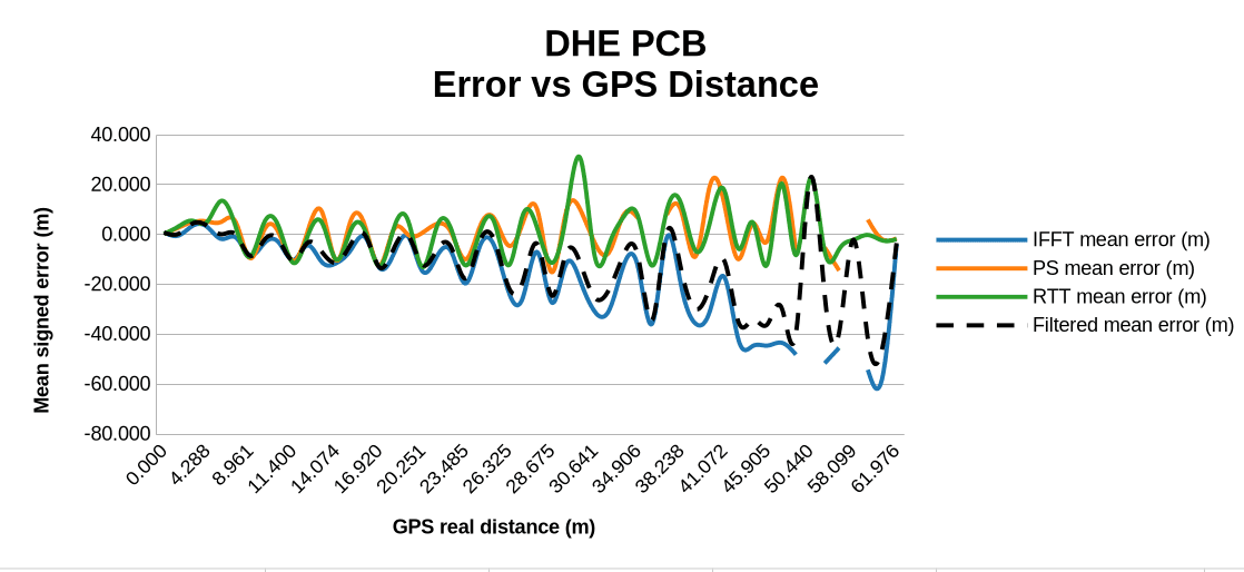
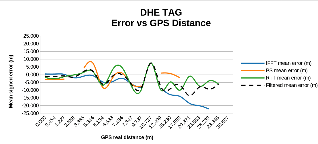
For both antenna profiles, the error grows as the Reflector moves away from the Initiator. The farthest received record is not automatically a valid ranging result: the DK produced records up to 61.976 m and the Tag produced one GPS-aligned record at 30.607 m, but these distances only describe observed capture coverage.

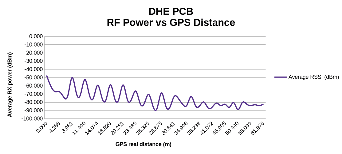
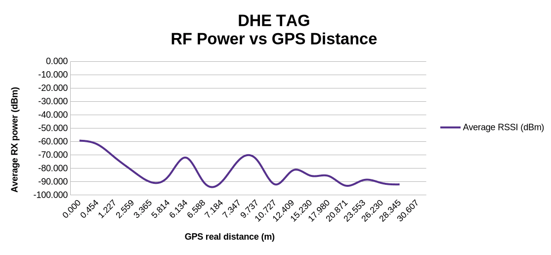
The following charts show the individual dynamic records after applying the CLOS calibration offsets. They illustrate how the error changes during motion, rather than a controlled average at a fixed distance.

Estimator Behavior

The DK CLOS calibration gives IFFT the largest fusion weight. In the dynamic data, IFFT became the least accurate estimator at longer distances, and its negative bias carried over into the filtered estimate, while RTT had the lowest standalone RMSE. This shows why fixed weights calculated in CLOS may not be the best approach for a changing environment.

Received RF Power vs. Distance

The RSSI trend follows the expected power loss with distance, but RSSI alone cannot tell you whether a measurement is reliable. The dynamic results show that signal power, agreement between estimators and availability must be considered together.

Conclusions

Bluetooth Channel Sounding gave us access to phase and timing information that let the application calculate distance with IFFT, Phase Slope and RTT. The tests also showed that these estimators are not independent of the antenna, the radio configuration or the environment. A calibration made for one antenna configuration could not be reused for another, and switching the Channel Sounding PHY to coded S8 required a new set of offsets and weights.

The CLOS campaign established those calibration values and showed how each estimator behaves on a controlled propagation path. The PCB antenna had lower residual error during calibration, which gave IFFT the highest fusion weight; the Tag had higher residual error and more balanced weights. These remain calibration results: removing the average bias in CLOS does not remove the error introduced later by body blockage, multipath or changes in the radio channel.

The body-blocking, static harsh and dynamic harsh tests showed this limitation clearly. Availability fell well below the 5 Hz reference rate in every non-CLOS scenario, and received power generally dropped as distance and obstruction increased. In the dynamic DK data, IFFT, the estimator with the largest fixed CLOS weight, had the largest long-distance error, so the filtered estimate inherited part of its negative bias, while RTT had the lowest standalone RMSE.

Bluetooth Channel Sounding is excellent for measuring distance with little interference, but its quality drops significantly in harsh environments, with growing error and lower availability. The application can compensate with statistical methods and adaptive, variance-dependent filtering.

What This Means for Your Product

If you are planning a product that relies on Bluetooth Channel Sounding (a digital key, an asset tag, a proximity feature or an indoor positioning system), these results point to a few practical steps:

• Calibrate per antenna and per radio configuration. Offsets measured on a development kit will not carry over to your final PCB, enclosure or PHY settings.

• Treat availability as a requirement. In our tests, 20–70% of 5 Hz slots produced a distance. Define the update rate your feature really needs and design filtering and UX around missing measurements.

• Don't rely on fixed fusion weights. Weights tuned in line of sight made the moving, real-world result worse. Adapt the weighting to estimator variance and agreement at run time.

• Judge quality by more than RSSI. Combine signal power, estimator agreement and availability to decide whether a distance can be trusted.

• Test where the product will live. Body blocking, crowds and metal changed the results far more than distance alone.

iomico's embedded team builds firmware on Nordic SoCs with Zephyr and the nRF Connect SDK, along with the hardware and antenna design around them. If you need help evaluating or integrating Bluetooth Channel Sounding, see our firmware development, Zephyr development and hardware design services, or read more about wireless options in IoT Connectivity: LoRaWAN, 5G and Nordic NR+ and DECT NR+ in Smart Street Lighting.

Planning to design and develop a product with Bluetooth Channel Sounding? Feel free to reach out to iomico for a consultation. We can help you choose the hardware, calibrate the ranging and test it in the conditions where your product will be used.

FAQ

How accurate is Bluetooth Channel Sounding?

In our nRF54L15 tests, accuracy depended on the environment more than on anything else. In clear line of sight, after per-antenna calibration, the average error of the fused estimate was 2 cm (DK) and 14 cm (Tag). On a busy street with static devices, RMSE was about 2–3 m at 3–10 m. With a moving device in the same street, error grew with distance and exceeded 25 m RMSE beyond 30 m for the DK.

Does the human body affect Bluetooth Channel Sounding?

Yes. On the DK, average received power fell from −76.6 dBm with only the Reflector blocked to −87.8 dBm with both devices blocked, and availability dropped to 20.6%. The line-of-sight calibration did not fully compensate for the added error.

Do you need to calibrate Bluetooth Channel Sounding?

Yes. Each estimator showed a systematic offset that depended on the antenna and the radio configuration (for example, 0.6–2.9 m on the DK and 0.9–5.6 m on the Tag), and a calibration made for one configuration could not be reused for another.

Is RSSI enough to judge whether a distance is reliable?

No. Received power fell with distance as expected, but it did not fully explain the error. Signal power, agreement between estimators and availability should be evaluated together.